1 Overview
Data warehouses such as Google BigQuery and Amazon RedShift allow you to create a data repository in which the data are structured like in a database (tables, fields, etc.), stored in the cloud, and queried efficiently (and in parallel) using the cloud provider’s infrastructure. Storage is by column, which allows for efficient queries when doing queries operating on large portions of tables.
BigQuery has some nice advantages over RedShift for one-off analyses (as opposed to regular, repeated operations). In particular, it requires less configuration/administration. BigQuery is ‘serverless’. Instead of you having to set up virtual machines to do the queries, BigQuery automatically sets up the computational resources for your query, scaled as appropriate for the size of the query.
Some features of BigQuery include:
- You can manage access to your datasets for different GCP users.
- You can query publicly available datasets.
- You can query “external tables” to access data not in a BigQuery dataset.
2 Running queries
Let’s first demonstrate running an SQL query in BigQuery. We’ll use a publicly available dataset. You can process your first one terabyte of data per month for free (that sounds like a lot, but queries can add up quickly when datasets are gigatyes in size or larger).
2.1 Using the BigQuery browser-based interface
These next instructions assume you have a Google Cloud Platform account with billing set up (e.g., using a credit card). To use the BigQuery Sandbox, see below.
Navigate to cloud.google.com and login (or create if needed) your Google
Cloud Platform account (which will be associated with your Google
account and its email address). Then go to the BiqQuery
website](https://console.cloud.google.com/bigquery) and click
Enable (if you haven’t enabled it previously for your account).
Now we can start working with BigQuery. The demo here follows these instructions.
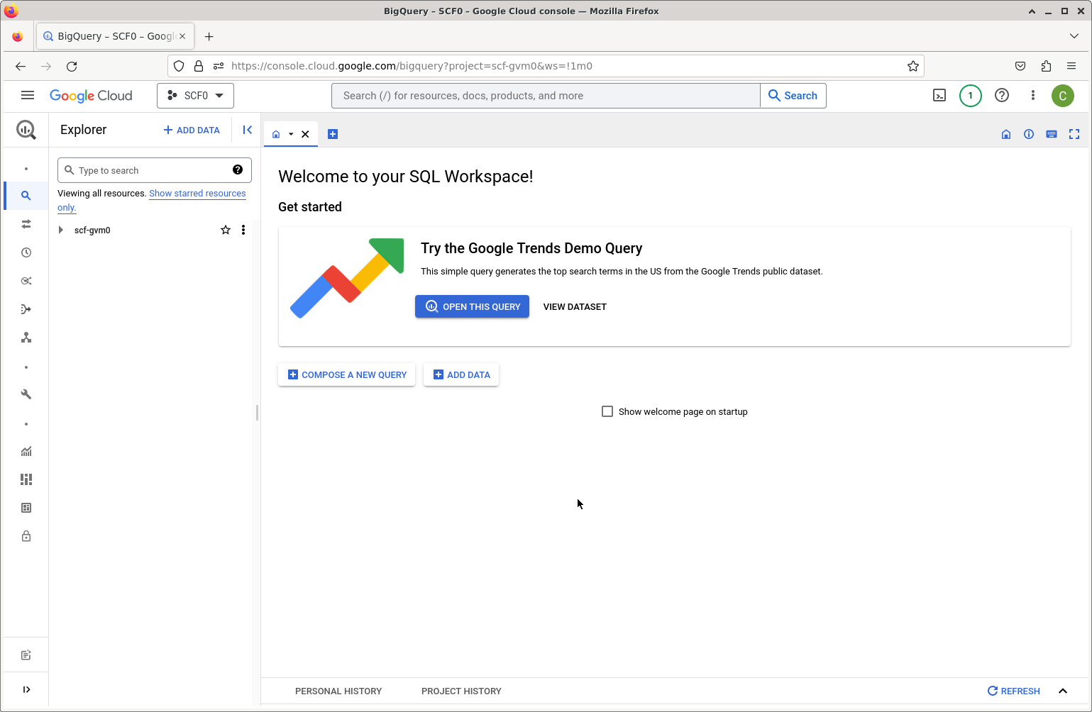
To use a public dataset, we’ll choose Add Data and scroll down to
Public Datasets. Search for “Stack Overflow”. Click on View Dataset.
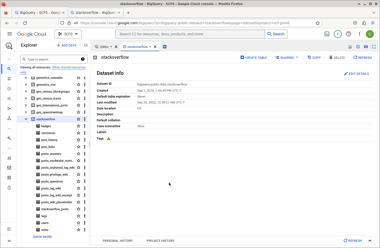
You’ll be able to see that the name of the dataset is
bigquery-public-data.stackoverflow. This dataset has similar data to
the Stack Overflow database used elsewhere in this tutorial, but the
schema differs somewhat.
In the Explorer pane you can search for “Stack Overflow” and be able
to view the tables, and then select tables to see the fields.
Now we can go to the Editor pane or select `Compose a New Query’ and
enter an SQL query.
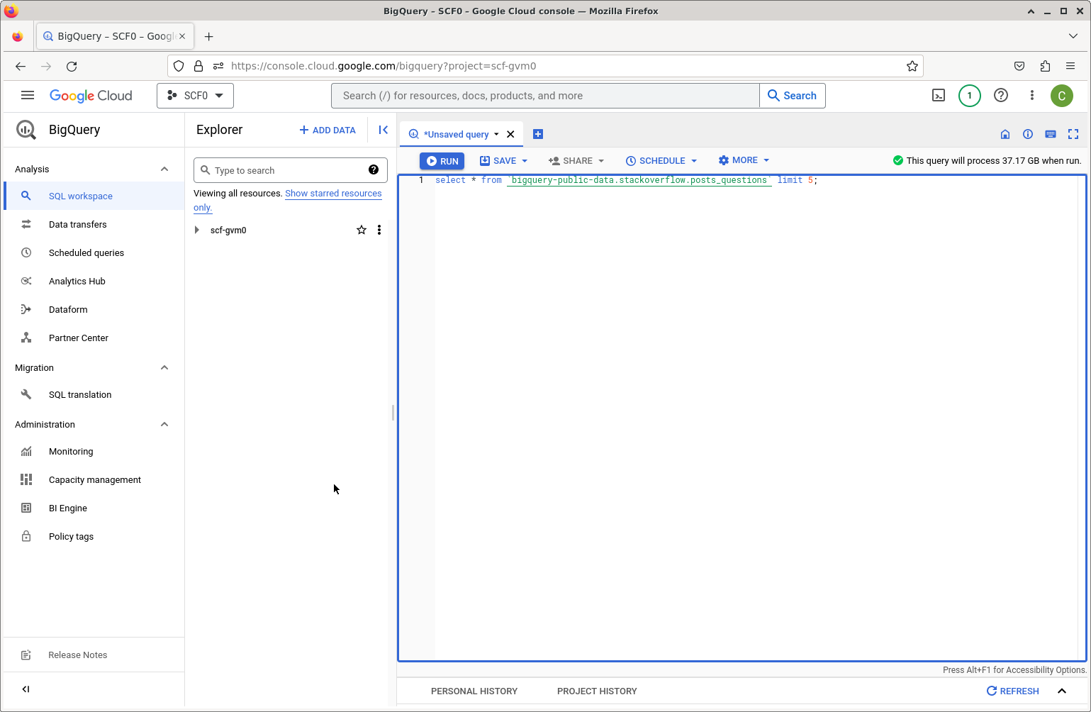
Note that BigQuery will preview how much data will be processed (see the upper right). Remember that you can process 1 TB for free each month.
This example query would process 37 GB. Maybe more of our free quota than we want to use at the moment.
select * from `bigquery-public-data.stackoverflow.posts_questions` limit 5;
This will only process 2.5 MB, so let’s run this:
select * from `bigquery-public-data.stackoverflow.tags` order by count desc limit 20;
The result (which you can see in the next section run from R) indicates
that javascript, python, java, and c# are the most popular tags.
You can save the results in various ways (to a local file, to Google Drive, as a BigQuery table, etc.
2.1.1 Using the free BigQuery Sandbox
You can use the Sandbox to avoid having to set up billing for your GCP account. The Sandbox has the same limits as BigQuery’s free tier, in particular 1 TB of processed query data each month.
Go to BigQuery, and login with your Google account. Set up a new project and then go to BigQuery and try it out (e.g., running the query above on the StackOverflow data).
2.2 Running queries from R or Python
2.2.1 Using R
We can use the bigrquery R package to interact with BigQuery from R
(e.g., running on a laptop).
myproject <- "some_project"
user <- "user@berkeley.edu"

library(bigrquery)
library(DBI)
The following will prompt for authentication to your Google account in a browser and save the authentication information as a ‘token’ associated with the email address.
If you’ve already done the authentication previously, it will reload the saved token, not requiring any interactivity, as done in generating this document.
bq_auth(email = user)
Now let’s connect to the public dataset and check the schema. To be able
to run queries, we need to be able to provide a GCP project that has
billing set up via the billing argument. It’s possible that the SQL
below would run if billing is set to be the name of a project without
billing set up (i.e., using the BigQuery Sandbox), but I haven’t checked
that.
drv <- bigquery()

db <- dbConnect(drv,
  project = "bigquery-public-data",
  dataset = "stackoverflow",
  billing = myproject
)

dbListTables(db)
##  [1] "badges"                     "comments"
##  [3] "post_history"               "post_links"
##  [5] "posts_answers"              "posts_moderator_nomination"
##  [7] "posts_orphaned_tag_wiki"    "posts_privilege_wiki"
##  [9] "posts_questions"            "posts_tag_wiki"
## [11] "posts_tag_wiki_excerpt"     "posts_wiki_placeholder"
## [13] "stackoverflow_posts"        "tags"
## [15] "users"                      "votes"
dbListFields(db, 'posts_questions')
##  [1] "id"                       "title"
##  [3] "body"                     "accepted_answer_id"
##  [5] "answer_count"             "comment_count"
##  [7] "community_owned_date"     "creation_date"
##  [9] "favorite_count"           "last_activity_date"
## [11] "last_edit_date"           "last_editor_display_name"
## [13] "last_editor_user_id"      "owner_display_name"
## [15] "owner_user_id"            "parent_id"
## [17] "post_type_id"             "score"
## [19] "tags"                     "view_count"
Now let’s run the simple query we tried before.
sql <- "select * from tags order by count desc limit 20"
dbGetQuery(db, sql)
## # A tibble: 20 × 5
##       id tag_name     count excerpt_post_id wiki_post_id
##    <int> <chr>        <int>           <int>        <int>
##  1     3 javascript 2426650         3624960      3607052
##  2    16 python     2026741         3624965      3607014
##  3    17 java       1866104         3624966      3607018
##  4     9 c#         1559412         3624962      3607007
##  5     5 php        1445747         3624936      3607050
##  6  1386 android    1386459         3625001      3607484
##  7     2 html       1146245         3673183      3673182
##  8   820 jquery     1029561         3625262      3607053
##  9    10 c++         776837         3624963      3606997
## 10     4 css         771867         3644670      3644669
## 11 58338 ios         674982         4536664      4536663
## 12    21 mysql       651413         3624969      3607033
## 13    22 sql         643145         3625226      3607304
## 14  4452 r           464242         3625322      3607736
## 15 46426 node.js     442811         4238969      4238968
## 16 92497 reactjs     415837        16880335     16880334
## 17   114 arrays      398827         4969094      4969093
## 18     8 c           385511         3624961      3607013
## 19    96 asp.net     370124         3625232      3607037
## 20  1508 json        346406         4889848      4889847
2.2.2 Using Python
We can use the Google BigQuery Python client
(package)
provided by Google. (We’ll also install the db-dtypes package so that
we convert the result of our query into a Pandas data frame.)
pip install google-cloud-bigquery db-dtypes
To authenticate, you’ll need to use the gcloud command line
interface. After installing that,
we run the authentication command.
gcloud auth application-default login
This will bring up a browser window and you can authenticate with your
Google account. It will save your credentials to a file in your home
directory, e.g., to
~/.config/gcloud/application_default_credentials.json. These
credentials will then be used by Google Cloud clients such as the
BigQuery client.
from google.cloud import bigquery
import db_dtypes  # needed for `to_dataframe()`

myproject <- "some_project"
db = bigquery.Client(project = myproject)

sql = "select * from bigquery-public-data.stackoverflow.tags order by count desc limit 20"
query_job = db.query(sql)  # API request
rows = query_job.result()  # Waits for query to finish

mydf = rows.to_dataframe()
mydf
The results (not shown) are the same as when done from R.
3 Getting data into BigQuery
Next, let’s demonstrate setting up a BigQuery data warehouse, using the Wikipedia data (used in the database management demos) as an example. Recall that we have data to populate a single table from multiple space-delimited flat text files, all of them in exactly the same format in terms of columns.
3.1 Loading a local file
We can load from a local file on our computer using Add Data, or we
can load from files already present in Google Cloud Storage.
First we’ll need to set IAM permissions on our account to allow the account to create and update tables.
To upload from a local file, select the Add Data button and choose the
file. There is no ‘space-separated’ file format, so we’ll choose CSV and
then in the advanced options, I need to specify that the delimiter is a
space using a “custom” field delimiter. You can choose to create a new
dataset. Since the files don’t have column names, I’ll choose to specify
the schema (the field names and types) in the Schema section of the
BigQuery form by clicking on the ‘+’ symbol to add each field,
specifically by entering this information: {date: string, maxlength = 8,
hour: string: maxlength = 6, site: string, page: string, count: integer,
size: numeric}.
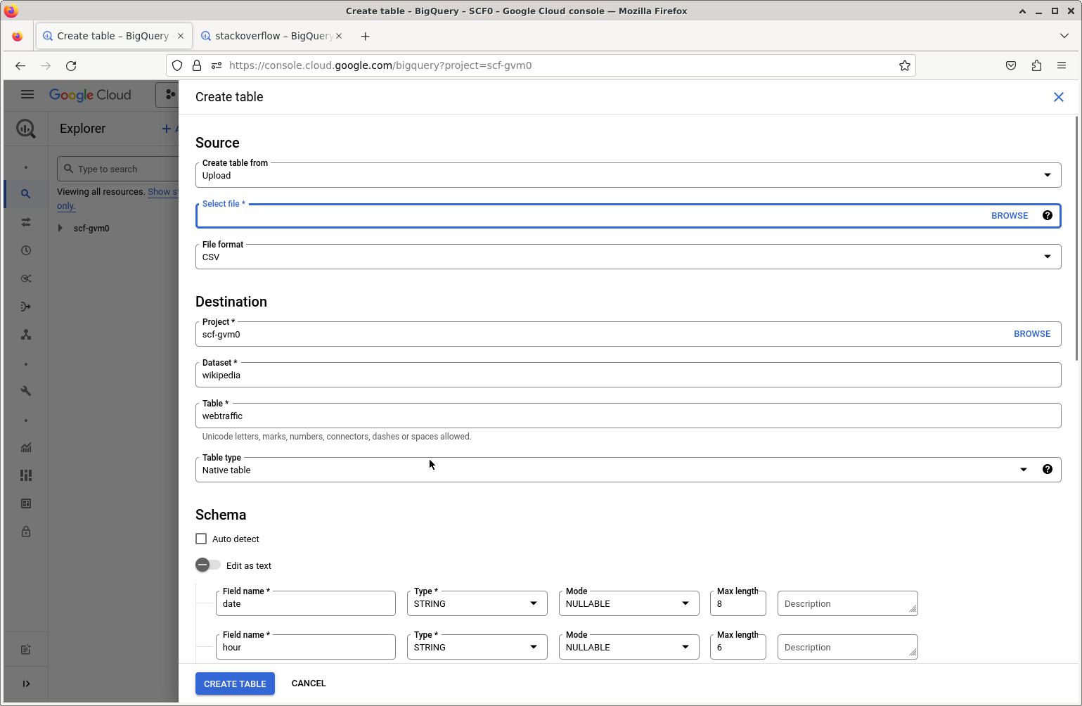
I’ll name the new BigQuery dataset wiki_test (this is equivalent to
the name of a database in a standard DBMS).
As was the case in the data management demos, we need to strip out double quote (“) symbols as BigQuery tries to interpret these as beginning and ending fields.
In the Add Data form, it looks like we can only add a single file at a
time, so for this test, I’ll just add one file.
Let’s see if we can now query the new table in the new dataset from R as done previously with the public Stack Overflow dataset.
db<- dbConnect(drv,
  project = myproject,
  dataset = "wiki_test",
  billing = myproject
)

dbListTables(db)
## [1] "webtraffic"
dbListFields(db, 'webtraffic')
## [1] "date" "hour" "site" "page" "count" "size"
Now let’s run a simple query:
sql <- "select * from webtraffic limit 5"
dbGetQuery(db, sql)
## # A tibble: 5 × 6
##   date     hour   site  page                        count   size
##   <chr>    <chr>  <chr> <chr>                       <int>  <dbl>
## 1 20081101 000001 af    Halloween                      12  94174
## 2 20081101 000001 af    Spesiaal:Onlangse_wysigings    25 360372
## 3 20081101 000001 af    Spesiaal:Search                50  52332
## 4 20081101 000001 af    Tempelhof-lughawe              26 115063
## 5 20081101 000001 af    Tuisblad                       33 514829
It worked!
3.2 Loading from Google Cloud Storage
Now let’s load multiple files all at once from Google Cloud Storage (GCS).
First we’ll take 10 of the files of the cleaned (no double quotes)
Wikipedia data and put them in GCS. Through the GCS web
interface, I’ll create a
bucket named wikipedia-cleaned-data and upload the files.
Now select Add Data in the BigQuery interface. We’ll select the source
as Google Cloud Storage, the file format as CSV (with the custom
separator of a space character) and use a “URI pattern” to select all 10
of the files: wikipedia-cleaned-data/part-*. We’ll name this dataset
wikipedia.
We can now run the same query as above on the new (larger) dataset:
db<- dbConnect(drv,
  project = myproject,
  dataset = "wikipedia",
  billing = myproject
)

dbListTables(db)
## [1] "webtraffic"
dbListFields(db, 'webtraffic')
## [1] "date" "hour" "site" "page" "count" "size"
Now let’s run a simple query:
sql <- "select * from webtraffic limit 5"
dbGetQuery(db, sql)
## # A tibble: 5 × 6
##   date     hour   site  page         count    size
##   <chr>    <chr>  <chr> <chr>        <int>   <dbl>
## 1 20081101 000001 fr    Psychose        15  295730
## 2 20081101 000001 fr    Skyrock_Blog    10  192848
## 3 20081101 000001 fr    Tunisie         36 3736262
## 4 20081101 000001 fr    Ulc%C3%A8re     10   60423
## 5 20081101 000001 fr    X_Japan         11  258634
3.3 Permissions
I did this using my Google Cloud account, which is an owner of the GCP account and so has various BigQuery permissions already set to allow various actions, including creating or modifying BigQuery datasets.
If you (as recommended) are using an IAM account, you are likely to need to set some permissions for the account to create or modify BigQuery datasets. In particular, as discussed here you need the following IAM permissions set:
- bigquery.tables.create
- bigquery.tables.updateData
- bigquery.tables.update
- bigquery.jobs.create
You can set these permissions by adding one of various IAM roles (e.g.,
roles/bigquery.dataEditor, roles/bigquery.dataOwner,
roles/bigquery.admin, bigquery.user, or bigquery.jobUser).