1 This Tutorial
This tutorial covers tools for manipulating large datasets, including those living in SQL databases or in data frames and related objects in R and Python. The focus is on querying rather than creating and administering databases as the intended audience is for statisticians/data analysts/data scientists who are carrying out analyses. A major emphasis is on how to do queries efficiently and how to use SQL effectively. At the moment, this tutorial is somewhat more focused on R than Python, but the manipulation of databases from R and Python are very similar because the core reliance is on SQL.
This tutorial assumes you have a working knowledge of R or Python.
1.1 Materials
Materials for this tutorial, including the Markdown files and associated
code files that were used to create these documents are available on
GitHub in the
gh-pages branch. You can download the files by doing a git clone from
a terminal window on a UNIX-like machine, as follows:
git clone https://github.com/berkeley-scf/tutorial-databases
The example data files are not part of the GitHub repository. You can get the example data files (both Stack Overflow data for 2021 and Wikipedia webtraffic data for the year 2008) here.
Solutions to the SQL challenges are available on request.
This tutorial by Christopher Paciorek of the UC Berkeley Statistical Computing Facility is licensed under a Creative Commons Attribution 3.0 Unported License.
1.2 Prerequisite Software
1.2.1 Using SQLite from R or Python
The simplest way to use a database is with SQLite, a lightweight database engine under which the database is stored simply in a single file.
Both R and Python can easily interact with an SQLite database. For R
you’ll need the RSQLite package. For Python you’ll need the sqlite3
package.
One thing to note is that SQLite does not have some useful functionality
that other databas management systems have. For example, you can’t use
ALTER TABLE to modify column types or drop columns.
1.2.2 DuckDB as a faster alternative to SQLite
DuckDB is another lightweight database engine under which the database is stored simply in a single file. It stores data column-wise, which can lead to big speedups when doing queries operating on large portions of tables (so-called “online analytical processing” (OLAP)).
Both R and Python can easily interact with a DuckDB database. For R
you’ll need the duckdb R package. For Python you’ll need the duckdb
Python package.
1.2.3 Using PostgreSQL on Mac or Windows
To replicate the (non-essential) PostgreSQL administration portion of this tutorial, you’ll need access to a machine on which you can run a PostgreSQL server. While there are a variety of ways to do this, this tutorial assumes that you are running PostgreSQL on an Ubuntu (or Debian) Linux machine. If you are a Windows or Mac user, there are several options for accessing a Linux environment:
- You could run Ubuntu in a Docker container; Docker can be installed on Windows or Mac. Once you’ve installed Docker and have access to a terminal command line, please see the commands in docker.sh in this repository.
- You could run an Amazon EC2/Google Cloud/Azure virtual machine instance, using a image that supports R and/or Python and then installing PostgreSQL as discussed in this tutorial.
- The big cloud computing providers have created a wide array of specific database services, so if you are using a cloud provider, you’d probably want to take advantage of those rather than ‘manually’ running a database via a virtual machine.
This tutorial by Christopher Paciorek is licensed under a Creative Commons Attribution 3.0 Unported License (CC BY).
2 Background
2.1 Data size
The techniques and tools discussed here are designed for datasets in the range of gigabytes to tens of gigabytes, though they may scale to larger if you have a machine with a lot of memory or simply have enough disk space and are willing to wait. If you have 10s of gigabytes of data, you’ll be better off if your machine has 10s of GBs of memory, as discussed in this tutorial.
If you’re scaling to 100s of GBs, terabytes or petabytes, using the cloud computing providers’ tools for working with big datasets is probably your best bet (e.g., Amazon RedShift or Google BigQuery), or possibly carefully-administered databases. Those topics are beyond the scope of this tutorial. However, this tutorial will be useful if you’re doing SQL queries on professionally-administered databases or databases in the cloud or in a Spark context.
2.2 Memory vs. disk
On a computer there is a hierarchy of locations where data can be stored. The hierarchy has the trade-off that the locations that the CPU can access most quickly can store the least amount of data. The hierarchy looks like this:
- cpu cache
- main memory
- disk
- local network (data stored on other machines)
- general internet access
For our purposes here the key question is whether the data resides in memory or on disk, but when considering Spark and distributed systems, one gets into issues of moving data across the network between machines.
Formally, databases are stored on disk, while R and Python store datasets in memory. This would suggest that databases will be slow to access their data but will be able to store more data than can be loaded into an R or Python session. However, databases can be quite fast due in part to disk caching by the operating system as well as careful implementation of good algorithms for database operations. For more information about disk caching see the database management document.
And conversely, R and Python have mechanisms for storing large datasets on disk in a way that they can be accessed fairly quickly.
3 Database systems and SQL
3.1 Overview of databases
Basically, standard SQL databases are relational databases that are a collection of rectangular format datasets (tables, also called relations), with each table similar to R or Pandas data frames, in that a table is made up of columns, which are called fields or attributes, each containing a single type (numeric, character, date, currency, enumerated (i.e., categorical), …) and rows or records containing the observations for one entity. Some of these tables generally have fields in common so it makes sense to merge (i.e., join) information from multiple tables. E.g., you might have a database with a table of student information, a table of teacher information and a table of school information.
One principle of databases is that if a set of fields contain duplicated information about a given category, you can more efficiently store information about each level of the category in a separate table. Consider information about people living in a state and information about each state - you don’t want to include variables that only vary by state in the table containing information about individuals (at least until you’re doing the actual analysis that needs the information in a single table). Or consider students nested within classes nested within schools.
Databases are set up to allow for fast querying and merging (called joins in database terminology).
You can interact with databases in a variety of database systems (DBMS=database management system). Some popular systems are SQLite, MySQL, PostgreSQL, Oracle and Microsoft Access. We’ll concentrate on accessing data in a database rather than management of databases. SQL is the Structured Query Language and is a special-purpose high-level language for managing databases and making queries. Variations on SQL are used in many different DBMS.
Queries are the way that the user gets information (often simply subsets of tables or information merged across tables). The result of an SQL query is in general another table, though in some cases it might have only one row and/or one column.
Many DBMS have a client-server model. Clients connect to the server, with some authentication, and make requests (i.e., queries).
There are often multiple ways to interact with a DBMS, including directly using command line tools provided by the DBMS or via Python or R, among others.
3.1.1 Relational Database Management Systems (DBMS)
There are a variety of relational database management systems (DBMS). Some that are commonly used by the intended audience of this tutorial are SQLite, PostgreSQL, and mySQL. We’ll concentrate on SQLite and DuckDB (because they are simple to use on a single machine) and PostgreSQL (because is is a popular open-source DBMS that is a good representative of a client-server model and has some functionality that SQLite lacks).
3.1.2 Serverless DBMS
SQLite and DuckDB are quite nice in terms of being self-contained - there is no server-client model, just a single file on your hard drive that stores the database. There is no database process running on the computer; rather SQLite or DuckDB are embedded within the host process (e.g., Python or R). (There are also command line interfaces (CLI) for both SQLite and DuckDB that you can start from the command line/terminal.)
3.1.3 NoSQL databases
NoSQL (not only SQL) systems have to do with working with datasets that are not handled well in traditional DBMS, and not specifically about the use or non-use of SQL itself. In particular data might not fit well within the rectangular row-column data model of one or more tables in a database. And one might be in a context where a full DBMS is not needed. Or one might have more data or need faster responses than can be handled well by standard DBMS.
While these systems tend to scale better, they generally don’t have a declarative query language so you end up having to do more programming yourself. For example in the Stanford database course referenced at the end of this tutorial, the noSQL video gives the example of web log data that records visits to websites. One might have the data in the form of files and not want to go through the trouble of data cleaning and extracting fields from unstructured text. In addition, one may need to do only simple queries that involve looking at each record separately and therefore can be easily done in parallel, which noSQL systems tend to be designed to do. Or one might have document data, such as Wikipedia pages, where the unstructured text on each page is not really suited for a DBMS.
Some NoSQL systems include
- Hadoop/Spark-style MapReduce systems,
- key-value storage systems (e.g., with data stored as pairs of keys (i.e., ids) and values, such as in JSON),
- document storage systems (like key-value systems but where the value is a document), and
- graph storage systems (e.g., for social networks).
3.2 Databases in the cloud
The various big cloud computing providers (AWS, Google Cloud Platform (GCP), Azure) provide a dizzying array of different database-like services. Here are some examples.
- Online database hosting services allow you to host databases (e.g., PostgreSQL databases) the infrastructure of a cloud provider. You basically manage the database in the cloud instead of on a physical machine. One example is Google Cloud SQL.
- Data warehouses such as Google BigQuery and Amazon RedShift allow you to create a data repository in which the data are structured like in a database (tables, fields, etc.), stored in the cloud, and queried efficiently (and in parallel) using the cloud provider’s infrastructure). Storage is by column, which allows for efficient queries when doing queries operating on large portions of tables.
- Data lakes store data in a less structured way in cloud storage in files (e.g., CSV, Parquet, Arrow, etc.) that generally have common structure. The data can be queried without creating an actual database or data warehouse.
Google’s BigQuery has the advantages of not requiring a lot of administration/configuration while allowing your queries to take advantage of a lot of computing power. BigQuery will determine how to run a query in parallel across multiple (virtual) cores. You can see a demonstration of BigQuery.
3.3 SQL
SQL is a declarative language that tells the database system what results you want. The system then parses the SQL syntax and determines how to implement the query.
Later we’ll introduce a database of Stack Overflow questions and answers.
Here is a simple query that selects the first five rows (and all
columns, based on the * wildcard) from a table (called ‘questions’) in
a database that one has connected to:
select * from questions limit 5
4 Schema and normalization
To truly leverage the conceptual and computational power of a database you’ll want to have your data in a normalized form, which means spreading your data across multiple tables in such a way that you don’t repeat information unnecessarily.
The schema is the metadata about the tables in the database and the fields (and their types) in those tables.
Let’s consider this using an educational example. Suppose we have a school with multiple teachers teaching multiple classes and multiple students taking multiple classes. If we put this all in one table organized per student, the data might have the following fields:
- student ID
- student grade level
- student name
- class 1
- class 2
- …
- class n
- grade in class 1
- grade in class 2
- …
- grade in class n
- teacher ID 1
- teacher ID 2
- …
- teacher ID n
- teacher department 1
- teacher department 2
- …
- teacher department n
- teacher age 1
- teacher age 2
- …
- teacher age n
There are a lot of problems with this.
- ‘n’ needs to be the maximum number of classes a student might take. If one ambitious student takes many classes, there will be a lot of empty data slots.
- All the information about individual teachers (department, age, etc.) is repeated many times, meaning we use more storage than we need to.
- If we want to look at the data on a per teacher basis, this is very poorly organized for that.
- If one wants to change certain information (such as the age of a teacher) one needs to do it in many locations, which can result in errors and is inefficient.
It would get even worse if there was a field related to teachers for which a given teacher could have multiple values (e.g., teachers could be in multiple departments). This would lead to even more redundancy - each student-class-teacher combination would be crossed with all of the departments for the teacher (so-called multivalued dependency in database theory).
An alternative organization of the data would be to have each row represent the enrollment of a student in a class, with as many rows per student as the number of classes the student is taking.
- student ID
- student name
- class
- grade in class
- student grade level
- teacher ID
- teacher department
- teacher age
This has some advantages relative to our original organization in terms of not having empty data slots, but it doesn’t solve the other three issues above.
Instead, a natural way to order this database is with the following tables.
- Student
- ID
- name
- grade_level
- Teacher
- ID
- name
- department
- age
- Class
- ID
- topic
- class_size
- teacher_ID
- ClassAssignment
- student_ID
- class_ID
- grade
Then we do queries to pull information from multiple tables. We do the joins based on ‘keys’, which are the fields in each table that allow us to match rows from different tables.
(That said, if all anticipated uses of a database will end up recombining the same set of tables, we may want to have a denormalized schema in which those tables are actually combined in the database. It is possible to be too pure about normalization! We can also create a virtual table, called a view, as discussed later.)
4.1 Keys
A key is a field or collection of fields that give(s) a unique value for every row/observation. A table in a database should then have a primary key that is the main unique identifier used by the DBMS. Foreign keys are columns in one table that give the value of the primary key in another table. When information from multiple tables is joined together, the matching of a row from one table to a row in another table is generally done by equating the primary key in one table with a foreign key in a different table.
In our educational example, the primary keys would presumably be: Student.ID, Teacher.ID, Class.ID, and for ClassAssignment two fields: {ClassAssignment.studentID, ClassAssignment.class_ID}.
Some examples of foreign keys would be:
- student_ID as the foreign key in ClassAssignment for joining with Student on Student.ID
- teacher_ID as the foreign key in Class for joining with Teacher based on Teacher.ID
- class_ID as the foreign key in ClassAssignment for joining with Class based on Class.ID
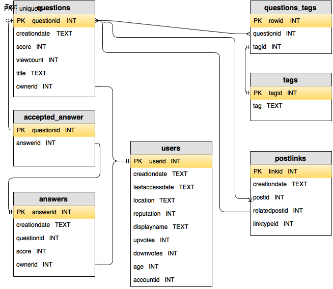
5 Stack Overflow example database
I’ve obtained data from Stack Overflow, the popular website for asking coding questions, and placed it into a normalized database. We’ll explore SQL functionality using this example database, which has metadata (i.e., it lacks the actual text of the questions and answers) on all of the questions and answers posted in 2021.
Let’s consider the Stack Overflow data. Each question may have multiple answers and each question may have multiple (topic) tags.
If we tried to put this into a single table, the fields could look like this if we have one row per question:
- question ID
- ID of user submitting question
- question title
- tag 1
- tag 2
- …
- tag n
- answer 1 ID
- ID of user submitting answer 1
- answer 2 ID
- ID of user submitting answer 2
- …
or like this if we have one row per question-answer pair:
- question ID
- ID of user submitting question
- question title
- tag 1
- tag 2
- …
- tag n
- answer ID
- ID of user submitting answer
As we’ve discussed neither of those schema is particularly desirable.
Question: How would you devise a schema to normalize the data. I.e., what set of tables do you think we should create?
Don’t peek until after you’ve thought about it, but you can view one reasonable schema here. The lines between tables indicate the relationship of foreign keys in one table to primary keys in another table. The schema in the actual databases of Stack Overflow data we’ll use in this tutorial is similar to but not identical to that.
5.1 Getting the database
You can download a copy of the SQLite version of the Stack Overflow database (only data for the year 2021) from here as part of the overall zip with all of the example datasets as discussed in the introduction of this tutorial.
In the next section I’ll assume the .db file is placed in the
subdirectory of the repository called data.
Note that all of the code used to download the data from the Stack
Overflow website and to manipulate it to create a complete Postgres
database and (for the year 2021 only) an SQLite database and CSVs for
each table is in the data/prep_stackoverflow
subdirectory
of this repository. Note that as of February 2022, the data are still
being kept up to date
online.
6 Accessing a database and using SQL from other languages
Although DBMS have their own interfaces (we’ll see a bit of this later), databases are commonly accessed from other programs. For data analysts this would often be Python or R, as seen next.
Most of our examples of making SQL queries on a database will be done from R, but they could just as easily have been done from Python or other programs.
6.1 Using SQL from R
The DBI package provides a front-end for manipulating databases from a variety of DBMS (SQLite, DuckDB, MySQL, PostgreSQL, among others). Basically, you tell the package what DBMS is being used on the back-end, link to the actual database, and then you can use the standard functions in the package regardless of the back-end.
With SQLite and DuckDB, R processes make calls against the stand-alone SQLite database (.db or .duckdb) file, so there are no SQLite-specific processes. With PostgreSQL, R processes call out to separate Postgres processes; these are started from the overall Postgres background process.
Apart from the different manner of connecting, all of the queries below are the same regardless of whether the back-end DBMS is SQLite, DuckDB, PostgreSQL, etc.
6.1.1 SQLite
You can access and navigate an SQLite database from R as follows.
library(RSQLite)
drv <- dbDriver("SQLite")
dir <- 'data' # relative or absolute path to where the .db file is
dbFilename <- 'stackoverflow-2021.db'
db <- dbConnect(drv, dbname = file.path(dir, dbFilename))
# simple query to get 5 rows from a table
dbGetQuery(db, "select * from questions limit 5")
##   questionid        creationdate score viewcount answercount
## 1   65534165 2021-01-01 22:15:54     0       112           2
## 2   65535296 2021-01-02 01:33:13     2      1109           0
## 3   65535910 2021-01-02 04:01:34    -1       110           1
## 4   65535916 2021-01-02 04:03:20     1        35           1
## 5   65536749 2021-01-02 07:03:04     0       108           1
##   commentcount favoritecount                               title
## 1            0            NA     Can't update a value in sqlite3
## 2            0            NA Install and run ROS on Google Colab
## 3            8             0       Operators on date/time fields
## 4            0            NA          Plotting values normalised
## 5            5            NA     Export C# to word with template
##    ownerid
## 1 13189393
## 2 14924336
## 3   651174
## 4 14695007
## 5 14899717
We can easily see the tables and their fields:
dbListTables(db)
## [1] "answers"        "questions"      "questions_tags"
## [4] "users"
dbListFields(db, "questions")
## [1] "questionid"    "creationdate"  "score"
## [4] "viewcount"     "answercount"   "commentcount"
## [7] "favoritecount" "title"         "ownerid"
dbListFields(db, "answers")
## [1] "answerid"     "questionid"   "creationdate" "score"
## [5] "ownerid"
One can either make the query and get the results in one go or make the
query and separately fetch the results. Here we’ve selected the first
five rows (and all columns, based on the * wildcard) and brought them
into R as a data frame.
results <- dbGetQuery(db, 'select * from questions limit 5')
class(results)
## [1] "data.frame"
query <- dbSendQuery(db, "select * from questions")
query
## <SQLiteResult>
##   SQL  select * from questions
##   ROWS Fetched: 0 [incomplete]
##        Changed: 0
results2 <- fetch(query, 5)
identical(results, results2)
## [1] TRUE
dbClearResult(query) # clear to prepare for another query
To disconnect from the database:
dbDisconnect(db)
6.1.2 DuckDB
You can access and navigate an DuckDB database from R as follows.
library(duckdb)
drv <- duckdb()
dir <- 'data' # relative or absolute path to where the .db file is
dbFilename <- 'stackoverflow-2021.duckdb'
dbd <- dbConnect(drv, file.path(dir, dbFilename))
# simple query to get 5 rows from a table
dbGetQuery(dbd, "select * from questions limit 5")
##   questionid            creationdate score viewcount answercount
## 1   65534165 2021-01-01T22:15:54.657     0       112           2
## 2   65535296 2021-01-02T01:33:13.543     2      1109           0
## 3   65535910 2021-01-02T04:01:34.137    -1       110           1
## 4   65535916 2021-01-02T04:03:20.027     1        35           1
## 5   65536749 2021-01-02T07:03:04.783     0       108           1
##   commentcount favoritecount                               title
## 1            0            NA     Can't update a value in sqlite3
## 2            0            NA Install and run ROS on Google Colab
## 3            8             0       Operators on date/time fields
## 4            0            NA          Plotting values normalised
## 5            5            NA     Export C# to word with template
##    ownerid
## 1 13189393
## 2 14924336
## 3   651174
## 4 14695007
## 5 14899717
To disconnect from the database:
dbDisconnect(dbd, shutdown = TRUE)
6.1.3 PostgreSQL
To access a PostgreSQL database instead, you can do the following, assuming the database has been created and you have a username and password that allow you to access the particular database.
library(RPostgreSQL)
drv <- dbDriver("PostgreSQL")
dbp <- dbConnect(drv, dbname = 'stackoverflow', user = 'paciorek', password = 'test')
# simple query to get 5 rows from a table, same as with SQLite:
dbGetQuery(dbp, "select * from questions limit 5")
6.2 Using SQL from Python
6.2.1 SQLite
import sqlite3 as sq
dir = 'data' # relative or absolute path to where the .db file is
dbFilename = 'stackoverflow-2021.db'
import os
db = sq.connect(os.path.join('data', dbFilename))
c = db.cursor()
c.execute("select * from questions limit 5")  # simple query
results = c.fetchall() # retrieve results
To disconnect:
c.close()
6.2.2 DuckDB
import duckdb
dir = 'data' # relative or absolute path to where the .duckdb file is
dbFilename = 'stackoverflow-2021.duckdb'
import os
db = duckdb.connect(os.path.join(dir, dbFilename))
db.sql("select * from questions limit 5")
6.2.3 PostgreSQL
import psycopg2 as pg
db = pg.connect("dbname = 'stackoverflow' user = 'paciorek' host = 'localhost' password = 'test'")
c = db.cursor()
7 References and Other Resources
In addition to various material found online, including various software manuals and vignettes, much of the SQL material was based on the following two sources:
- The Stanford online Introduction to Databases course (MOOC) released in Fall 2011, a version of which is available on edX.
- Harrison Dekker’s materials from a Statistics short course he taught in January 2016.
I’ve heard good things about the interactive exercises/tutorials at SQLZoo and the book Practical SQL by Anthony DeBarros (available through Berkeley’s library); in particular the first 200 or so pages (through chapter 12) cover general SQL programming/querying.